V. Classifier
Classifier allows you to train the computer to identify objects of interest by applying iterative, user-supervised machine learning methods to object measurements.
You first request (Fetch) object tiles (cropped from their original images), then manually sort them into classification bins (representing object classes), to form an annotated set. Once each bin contains several example objects, you can start training Classifier on the annotated set, i.e., asking the machine to learn how to differentiate the classes. Once Classifier is trained, you can continue training by fetching and sorting either more random objects or those objects that Classifier scores as being in a particular class; by fetching the objects predicted by Classifier to belong to a certain class and correcting errors in these classifications, subsequent Classifiers rapidly improve. Usually several rounds of refinement are necessary to train Classifier to recognize the classes of interest.
Once classification reaches a desirable accuracy, Classifier can “score” your experiment. This entails classifying all objects, counting how many objects of each class are in each image or group (if you have defined groups in your properties file; see section II.G), and computing the enrichment/depletion of each class per image or per group.
V.A Classifier quick-start guide
Launch Classifier and enter the number of objects you want Classifier to fetch.
Specify whether Classifier should select these objects from the entire experiment, a single image or a group, and whether it should apply any filters. Groups will only be available if defined in your properties file (section II).
Click Fetch. n distinct objects will appear in the unclassified bin.
Manually sort the unclassified objects into classification bins, adding additional bins if needed. Often, two bins are used: positive and negative. Bin names can be changed by right clicking empty space in the relevant bin.
Enter the number of top features you want to see (or if FastGentleBoosting is the chosen classifier, the maximum number of rules you want Classifier to look for). Click Train.
Repeat steps 2–5 to fetch and sort more objects. You will be able to specify that Classifier only retrieves objects that it deems to be in a particular class or objects that are difficult to classify so that you can correct errors.
Click Score Image to visualize object classifications in a particular image (you will be asked to enter an image ID number). Objects can be dragged and dropped into bins from the Image Viewer or Image Gallery for further training.
It is important to save the training set for future refinement, to re-generate scores, and as a record of your experiment. It is advisable to do so before proceeding to scoring your experiment since scoring may take a long time for large screens. Select File > Save Training Set from the menu bar (or
ctrl+S).Click Score All to have Classifier score your entire experiment (optionally with groups or filters). Classifier will present the results in a Table Viewer (described in section IV).
You can click on column headings to sort the data by that column, helping you identify images that are highly enriched in a given object class, or images that simply have a high count of those objects. You can double-click the headers of rows to view the corresponding images and then drag and drop objects from the resulting image(s) into classification bins to improve the classifier.
You can save Classifier’s scores for each image (or group) from the Table Viewer using File > Save data to CSV or Save per-image counts to CSV to create comma-separated value files. You can also view the scores with CPA’s visualization tool, Plate Viewer, by using Database > Write Temporary Table in Database and running the Plate Viewer (section IV).
V.B In-depth guidance for using Classifier
V.B.1 Configuring Classifier
Launch Classifier by clicking the Classifier icon in the CPA toolbar. The main Classifier screen will appear. If you have previously saved a training set, you can load it using File > Load Training Set:

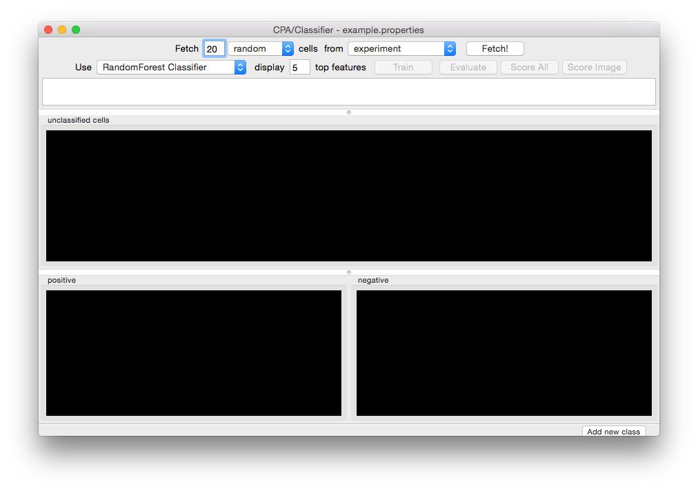
Initial Classifier screen.
Adding, Deleting, and Renaming Bins
Tip: Use as few bins as necessary for the relevant downstream analysis; adding too many bins can decrease the overall accuracy.
To add more bins at any time, click the Add new class button in the extreme lower right-hand corner of the window. You will see the Rename class popup window:
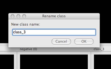
Adding a sorting bin.
Right-clicking inside any bin displays a popup menu that contains a number of options, including deleting and renaming bins. The remaining options in this menu apply to the contents of the 17 bin. See section III.C.3 for more information.
Right clicking on a sorting bin.
Adjusting the display
The menu bar at the top of the screen contains options for adjusting the display of the image tiles that will be displayed. View > Image Controls will bring up the same control panel found in the Image Viewer tool (section V), and the channel menus can be used to map different colors onto the respective channels. (Actin, pH3, and DNA, in this example; named so in the properties file as described in section II.)
Classifier menu bar.
V.B.2 Fetch an initial batch of objects
n distinct objects are fetched (retrieved) using the top portion of the main Classifier window:

Controls to fetch objects.
How many objects? Enter the number of distinct objects you want Classifier to fetch (default = 20)
Which class of objects should be retrieved? At this stage, random will be the only option available in the left-hand menu. After you Train Classifier (section III.C.5, following), new options will appear relating to each classification bin.
From which images? Two system-supplied default values in the right-hand menu are experiment and image. Select experiment to have Classifier retrieve objects from your entire experiment; select image to retrieve objects from a particular image (you will be asked to type its ID number). If you want to fetch objects from particular subsets of images in the experiment (e.g., control samples), you can set up filters by choosing the third default value in the right-hand menu create new filter; you can also define filters and groups of images in your properties file (described earlier in section II.G).
Click the Fetch button (located next to the right-hand menu) when you are ready to proceed, and you will see results like this:
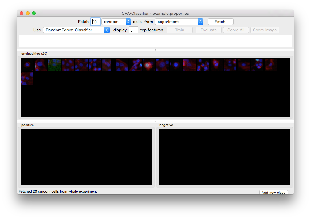
Twenty unclassified cells have been fetched and are ready for initial sorting.
V.B.3 Sort the initial batch of objects
Use your mouse to drag and drop object tiles into the classification bins you configured in step III.C.1. If you are uncertain about the classification of a particular object, it can be ignored or removed by selecting it and pushing the Delete key. Keep in mind, however, that classifier will ultimately score ALL objects found in your table unless you define filters to ignore certain images (see section II.F).
You can also sort objects into bins by using the arrow keys to select objects and the number keys 1-9 to assign objects into classes. Class bins are numbered left-to-right starting from 1.
Important: A small dot is displayed in the center of each tile as your mouse hovers over it. The
object that falls under this dot is the object that must be sorted. In the example below, the tile
under the mouse should be sorted based on the blue cell underneath the dot, NOT the cells
surrounding it. To change cropping size of the tile “window”, adjust the field image_tile_size in the properties file (section II.D).
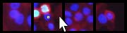
The object to be sorted is indicated by a small dot.
Once you have placed tiles in at least two bins, you have created Classifier’s initial training set, which will be used to train the classifier to differentiate objects in different classes.
Tip: Clicking on a tile will select it. Holding shift will allow you to add and remove tiles from the selection. All the tiles in a selection can be moved at once by dragging one of them to another bin.
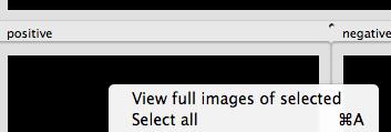
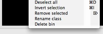
Some helpful tools are available when you right-click on a tile:
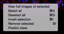
Right-clicking on a tile.
Select View full images of selected or double-click an individual tile to show the object in the context of the image from which it was drawn. This launches the Image Viewer tool (section V).
Tip: Objects can dragged and dropped from the Image Viewer or Image Gallery into class bins just as they are from the bins themselves. Use Shift+click to add/remove multiple objects to/from a selection, and ctrl+A/Ctrl+D to select/deselect all objects in the image.
Select all/Deselect all (
ctrl+A/ctrl+D) selects/deselects all tiles in the bin so they can be dragged and dropped together.Invert selection (
ctrl+I) to invert your selection (that is, select all non-selected tiles in the current bin and deselect all selected tiles).Remove selected (
Delete) removes the selected tiles from the current bin.Remove duplicates Right click on a bin to find this option. This will clear any duplicate tiles from the selected bin.
Selecting multiple tiles You can click on the bin background and drag the mouse to select multiple objects with a box.
V.B.4 Saving and loading training sets
Objects sorted into the bins are known as the training set. You can save the training set at any time, allowing you to close CPA and pick up where you left off later by re-loading the training set. Save and load training sets using File > Save training set or File > Load training set.
Warning: Loading a training set will cause all existing bins and tiles to be cleared.
V.B.5 Training Classifier
Continue repeating the process of fetching objects, sorting them into their appropriate classes, and training. Scoring (section III.C.6, following) can be used when you have finished creating a training set (that is, you are satisfied by its performance), but note that, as described later, scoring can also be used as another iterative step in creating the training set.
Assessing accuracy
The most accurate way to gauge Classifier’s performance is to fetch a large number of objects of a given class (e.g., positive) from the whole experiment. The fraction of the retrieved objects correctly matching the requested phenotype indicates the classifier’s general performance. For example, if you fetch 100 positive objects but find upon inspection that 5 of the retrieved objects are not positives, then you can expect Classifier to have a positive predictive value of 95% on individual cells (and similarly for negative predictive value in the case of two classes). Note that sensitivity, specificity, and negative and positive predictive values must be interpreted in the context of the actual prevalence of individual phenotypes, which may be difficult to assess a priori.
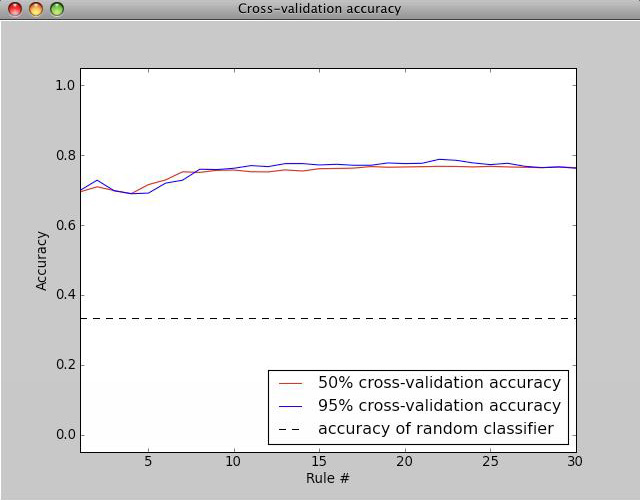
The Evaluate button calculates cross-validation metrics given the annotated set. Values closer to 1 indicate better performance. The cross-validation is 5 fold, and for each fold, the annotated set is split into a training and testing set (the split is stratified, meaning class proportions remain intact) and the algorithm is trained on the training set, then evaluated on the test set. To get final values, the evaluations are averaged over all folds. The evaluation can display a classification report, which is the recall, precision, and F1 score per class, or a confusion matrix, which is a matrix where the element in row i, column j has true class i and predicted class j.
Another way to gauge the classifier’s performance is to use the Score Image button on positive and negative controls (see the following section). Score Image allows you to see qualitatively how Classifier performs on a single image. Although the results cannot be reliably extrapolated to other images, it can be useful to examine control images and further refine the classifier by adding misclassified objects in those images to the proper bins.
The relationship between accuracy on individual cells versus performance scoring wells for follow-up is complicated, because false positive and false negatives are not evenly distributed throughout an experiment. In practice, improving accuracy on individual cells leads to better accuracy on wells, and in general, the accuracy on wells is better than the per-cell accuracy.
V.B.6 Scoring
Score image
Scoring a single image can be useful in several ways:
You can display an image and rapidly identify and correct classification errors in the image, by dragging and dropping objects from the image into bins.
You can use it as visual feedback to verify your classifier’s accuracy on a given image (especially a control image) at any point in the training process.
You can also use it to check Classifier’s classifications for individual images with unusual scores displayed in the Table Viewer produced by Score All (described in the next section).
To score a single image qualitatively, select Score Image and enter an image number. Classifier displays the image in Image Viewer (described in section V), with objects marked according to their classifications, based on the trained classifier. To save the resulting image as either a .jpg or .png file, select File > Save Image from the menu bar (or shortcut Ctrl+S).
Note
Note: This function is not yet capable of saving the classification markings.
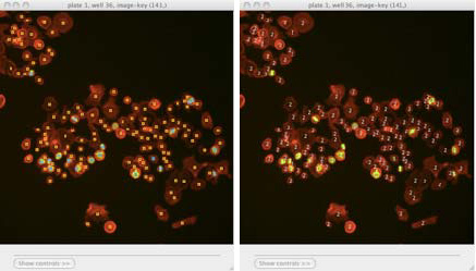
Scoring an image: Identifying classes by color (blue and yellow squares, left) and by number (right). Note that we have chosen to hide the blue channel (DNA stain) while viewing these images.
To display the object classes by number rather than color, select View > View object classes as numbers from the menu bar.
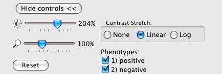
The Image Viewer control panel after scoring an image.
The brightness, contrast, and zoom controls work exactly as described for Image Viewer (section V). Note, however, the two checkboxes under Phenotypes: you can now select/deselect positive and negative results to display or hide only these objects in the image as requested.
Score all
Click Score All to classify all objects in your database using the current trained classifier. It can be helpful to score all images in the experiment and open some of the top-scoring images with Score Image to check classification accuracy. Training can be further refined by dragging and dropping objects from the image into bins in order to correct classification errors in images.
The result of Score All is a table of object counts and enrichment values for each classification you defined. You can then sort by these columns to find images (or groups, e.g., wells as collections of images) that are enriched or depleted for a particular classification, based on object counts or enrichment scores (see figure below for details).
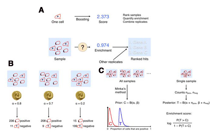
Description of enrichment score calculation. (A) While machine learning methods are used to produce per-cell scores, the challenge remains to model the sample distributions to generate a per-sample enrichment score. (B) Samples with varied positive/negative counts can be viewed as being drawn from a Beta distribution. (C) The full population is treated as independent samples to yield C = Beta(, ) which is used as the full-population-level prior for future observations. This prior is updated with new observations by computing the distribution of the positive fraction as the posterior T = Beta( + npos, + nneg), where npos and nneg are the positive and negative counts, respectively. The enrichment score for each sample is then calculated as the logit of P(T > C).
Note: Enrichment scores are computed for each sample as the logit area under the ROC curve for the prior versus the posterior distribution. The prior is computed from the full experiment using a Dirichlet-Multinomial distribution (a multi-class extension of Beta-Binomial) fit to the groups, and the posterior is computed for each group independently; that is, each phenotype is treated as positive and all others as negative for each phenotype in turn. - Tip: In most cases results should be ranked by enrichment score because this score takes into account both the number of objects in the class of interest as well as the total number of objects in the group.
If you have defined any groups or filters, you will have the option to select them here for use in scoring. If no groups or filters are defined, the window will contain only the default group Image and the default filter None.
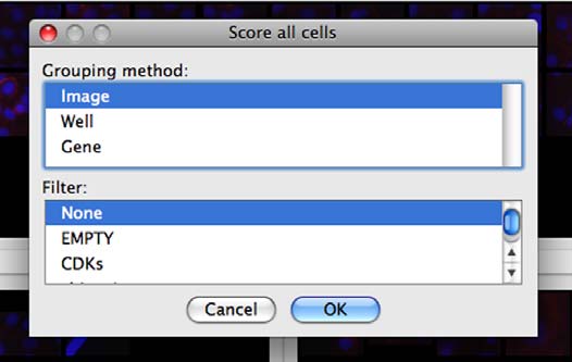
Classifier group/filter selection window.
Classifier presents its results in the Table Viewer tool, described in the next section. The table shows object counts and enrichment values for each phenotype you trained Classifier to recognize. To view this information graphically, return to the main Classifier screen and select Tools > Plate Viewer from the menu bar (see section VI for details).

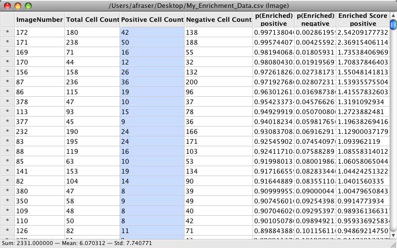
Enrichment Table Viewer produced by Classifier. Here we have grouped the counts and statistics on a per-image basis. We have ordered the data by the “Enriched Score Positive” column. The most highly enriched images were 172, 171, 169, and 170. With the “Positive Cell Count” column selected, we can see in the status bar that there are a total of 2331 positive cells in our experiment, with a mean of 6.07 positive cells per image, and a standard deviation of 7.74.
V.B.7 Data preparation
Typically one wouldn’t use the raw features as input for the machine learning, but the data is cleaned in some ways (e.g., by removing zero variance features) and normalized. Data preparation takes place before the machine learning is done, i.e., before training a classifier. We here describe how you can perform data preparation steps in CPA.
Scaling
Features can be normalised and centered before training/classification by activating the Scaler option in Advanced > Use Scaler. The features are centered to have mean 0 and scaled to have standard deviation 1
Normalization Tool
Outside the classifier scaling can be done with the Normalization Tool. From the main menu, navigate to Tools > Normalization Tool. You can choose which features to normalize and save the resulting table for later use.
Removing zero variance features
A zero variance feature is a feature that has the same entry for all objects, for example a feature that is equal to a constant value of 1 for all cells, which doesn’t provide information to classify the cells. Usually these features therefore are removed before training a classifier. You can analyze all zero variance features using Classifier->Advanced->Check features. Then either drop those features manually in the properties file or use the normalization tool to delete them.
Removing NANs
A standard procedure is finding features with NAN (not a number) entries in the data and removing those cells. CPA automatically ignores cells with NANs, so this step is already been taken take of.
V.B.8 Classifier types
CPA supports several different classifier types:
RandomForest: Produces a series of decision tree classifiers and uses averaging across all trees to generate predictions.
AdaBoost: Fits a series of weak learners (simple classification rules which don’t perform well alone). The input data is adjusted after each cycle to add weight to samples which the previous learner classified incorrectly. As learners are added, examples that are difficult to predict receive increasing influence. A final prediction is generated from a weighted majority vote from all learners.
SVC: Support Vector Classification. This technique considers all features and attempts to generate multi-dimensional dividing lines (termed “hyperplanes”) which will distinguish between classes.
GradientBoosting: This takes a similar approach to AdaBoost, but uses gradients instead of weights to make adjustments to the importance of individual samples.
LogisticRegression: Classifies objects via logistic regression. Classifications are made based on a series of curves corresponding to decision boundaries.
LDA: Linear Discriminant Analysis. This method projects the input data to a linear subspace consisting of the directions which maximize the separation between classes, then establishes a boundary which discriminates the classes.
KNeighbors: Classifies based on the majority class of the nearest k known samples. Classification is inferred from the training points nearest to the test sample.
FastGentleBoosting: A modification of the AdaBoost classification strategy, with optimisations for working with limited training data.
Neural Network: Generates a multi-layer perceptron neural network. Layers of neurons link each input feature to output features. Each neuron generates a signal based on it’s input and weighting from each source. The user can customise the number of intermediate ‘hidden’ layers between the input (measurement) and output (class) neurons. Additional hidden layers can help to generate more complex classifications. Neuron count per layer should generally be set to between the number of classes and number of input features.