Module: IdentifyPrimaryObjects

  The units used here are pixels so that it is easy to zoom in on objects and determine typical diameters. To measure distances in an open image, use the "Measure length" tool under Tools in the display window menu bar. If you click on an image and drag, a line will appear between the two endpoints, and the distance between them shown at the right-most portion of the bottom panel.

A few important notes:

• Several other settings make use of the minimum object size entered here, whether the Discard objects outside the diameter range? setting is used or not:
  • Automatically calculate size of smoothing filter for declumping?
  • Automatically calculate minimum allowed distance between local maxima?
  • Automatically calculate the size of objects for the Laplacian of Gaussian filter? (shown only if Laplacian of Gaussian is selected as the declumping method)
• For non-round objects, the diameter here is actually the "equivalent diameter", i.e., the diameter of a circle with the same area as the object.

Objects discarded based on size are outlined in magenta in the module's display. See also the FilterObjects module to further discard objects based on some other measurement.

  Select Yes allows you to exclude small objects (e.g., dust, noise, and debris) or large objects (e.g., large clumps) if desired.

This is helpful in cases when an object was incorrectly split into two objects, one of which is actually just a tiny piece of the larger object. However, this could be problematic if the other settings in the module are set poorly, producing many tiny objects; the module will take a very long time trying to merge the tiny objects back together again; you may not notice that this is the case, since it may successfully piece together the objects again. It is therefore a good idea to run the module first without merging objects to make sure the settings are reasonably effective.

  Removing objects that touch the image border is useful when you do not want to make downstream measurements of objects that are not fully within the field of view. For example, morphological measurements obtained from a portion of an object would not be accurate.

Objects discarded due to border touching are outlined in yellow in the module's display. Note that if a per-object thresholding method is used or if the image has been previously cropped or masked, objects that touch the border of the cropped or masked region may also discarded.

• The pixel intensities of the input image (this is the most common).
• A single value manually provided by the user.
• A single value produced by a prior module measurement.
• A binary image (called a mask) where some of the pixel intensity values are set to 0, and others are set to 1.

• Automatic: Use the default settings for thresholding. This strategy calculates the threshold using the MCT method on the whole image (see below for details on this method) and applies the threshold to the image, smoothed with a Gaussian with sigma of 1.

    This approach is fairly robust, but does not allow you to select the threshold algorithm and does not allow you to apply additional corrections to the threshold.

• Global: Calculate a single threshold value based on the unmasked pixels of the input image and use that value to classify pixels above the threshold as foreground and below as background.

    This strategy is fast and robust, especially if the background is uniformly illuminated.

• Adaptive: Partition the input image into tiles and calculate thresholds for each tile. For each tile, the calculated threshold is applied only to the pixels within that tile.
  

    This method is slower but can produce better results for non-uniform backgrounds. However, for signifcant illumination variation, using the CorrectIllumination modules is preferable.

• Per object: Use objects from a prior module such as IdentifyPrimaryObjects to define the region of interest to be thresholded. Calculate a separate threshold for each object and then apply that threshold to pixels within the object. The pixels outside the objects are classified as background.

    This method can be useful for identifying sub-cellular particles or single-molecule probes if the background intensity varies from cell to cell (e.g., autofluorescence or other mechanisms).

• Manual: Enter a single value between zero and one that applies to all cycles and is independent of the input image.

    This approach is useful if the input image has a stable or negligible background, or if the input image is the probability map output of the ClassifyPixels module (in which case, a value of 0.5 should be chosen). If the input image is already binary (i.e., where the foreground is 1 and the background is 0), a manual value of 0.5 will identify the objects.

• Binary image: Use a binary image to classify pixels as foreground or background. Pixel values other than zero will be foreground and pixel values that are zero will be background. This method can be used to import a ground-truth segmentation created by CellProfiler or another program.

    The most typical approach to produce a binary image is to use the ApplyThreshold module (image as input, image as output) or the ConvertObjectsToImage module (objects as input, image as output); both have options to produce a binary image. It can also be used to create objects from an image mask produced by other CellProfiler modules, such as Morph. Note that even though no algorithm is actually used to find the threshold in this case, the final threshold value is reported as the Otsu threshold calculated for the foreground region.

• Measurement: Use a prior image measurement as the threshold. The measurement should have values between zero and one. This strategy can be used to apply a pre-calculated threshold imported as per-image metadata via the Metadata module.

    Like manual thresholding, this approach can be useful when you are certain what the cutoff should be. The difference in this case is that the desired threshold does vary from image to image in the experiment but can be measured using another module, such as one of the Measure modules, ApplyThreshold or an Identify module.

Both the automatic and manual options have advantages and disadvantages.

  An automatically-calculated threshold adapts to changes in lighting/staining conditions between images and is usually more robust/accurate. In the vast majority of cases, an automatic method is sufficient to achieve the desired thresholding, once the proper method is selected.

In contrast, an advantage of a manually-entered number is that it treats every image identically, so use this option when you have a good sense for what the threshold should be across all images. To help determine the choice of threshold manually, you can inspect the pixel intensities in an image of your choice. To view pixel intensities in an open image, use the pixel intensity tool which is available in any open display window. When you move your mouse over the image, the pixel intensities will appear in the bottom bar of the display window..

  The manual method is not robust with regard to slight changes in lighting/staining conditions between images.

The automatic methods may ocasionally produce a poor threshold for unusual or artifactual images. It also takes a small amount of time to calculate, which can add to processing time for analysis runs on a large number of images.

The threshold that is used for each image is recorded as a per-image measurement, so if you are surprised by unusual measurements from one of your images, you might check whether the automatically calculated threshold was unusually high or low compared to the other images. See the FlagImage module if you would like to flag an image based on the threshold value.

There are a number of methods for finding thresholds automatically:

• Otsu: This approach calculates the threshold separating the two classes of pixels (foreground and background) by minimizing the variance within the each class.

    This method is a good initial approach if you do not know much about the image characteristics of all the images in your experiment, especially if the percentage of the image covered by foreground varies substantially from image to image.

    Our implementation of Otsu's method allows for assigning the threhsold value based on splitting the image into either two classes (foreground and background) or three classes (foreground, mid-level, and background). See the help below for more details.

• Mixture of Gaussian (MoG):This function assumes that the pixels in the image belong to either a background class or a foreground class, using an initial guess of the fraction of the image that is covered by foreground.

    If you know that the percentage of each image that is foreground does not vary much from image to image, the MoG method can be better, especially if the foreground percentage is not near 50%.

    This method is our own version of a Mixture of Gaussians algorithm (O. Friman, unpublished). Essentially, there are two steps:

  1. First, a number of Gaussian distributions are estimated to match the distribution of pixel intensities in the image. Currently three Gaussian distributions are fitted, one corresponding to a background class, one corresponding to a foreground class, and one distribution for an intermediate class. The distributions are fitted using the Expectation-Maximization algorithm, a procedure referred to as Mixture of Gaussians modeling.
  2. When the three Gaussian distributions have been fitted, a decision is made whether the intermediate class more closely models the background pixels or foreground pixels, based on the estimated fraction provided by the user.

• Background: This method simply finds the mode of the histogram of the image, which is assumed to be the background of the image, and chooses a threshold at twice that value (which you can adjust with a Threshold Correction Factor; see below). The calculation includes those pixels between 2% and 98% of the intensity range.

    This thresholding method is appropriate for images in which most of the image is background. It can also be helpful if your images vary in overall brightness, but the objects of interest are consistently N times brighter than the background level of the image.

• RobustBackground: Much like the Background: method, this method is also simple and assumes that the background distribution approximates a Gaussian by trimming the brightest and dimmest 5% of pixel intensities. It then calculates the mean and standard deviation of the remaining pixels and calculates the threshold as the mean + 2 times the standard deviation.

    This thresholding method can be helpful if the majority of the image is background, and the results are often comparable or better than the Background method.

• RidlerCalvard: This method is simple and its results are often very similar to Otsu. RidlerCalvard chooses an initial threshold and then iteratively calculates the next one by taking the mean of the average intensities of the background and foreground pixels determined by the first threshold. The algorithm then repeats this process until the threshold converges to a single value.

    This is an implementation of the method described in Ridler and Calvard, 1978. According to Sezgin and Sankur 2004, Otsu's overall quality on testing 40 nondestructive testing images is slightly better than Ridler's (average error: Otsu, 0.318; Ridler, 0.401).

• Kapur: This method computes the threshold of an image by searching for the threshold that maximizes the sum of entropies of the foreground and background pixel values, when treated as separate distributions.

    This is an implementation of the method described in Kapur et al, 1985.

• Maximum correlation thresholding (MCT): This method computes the maximum correlation between the binary mask created by thresholding and the thresholded image and is somewhat similar mathematically to Otsu.

    The authors of this method claim superior results when thresholding images of neurites and other images that have sparse foreground densities.

    This is an implementation of the method described in Padmanabhan et al, 2010.

References

• Sezgin M, Sankur B (2004) "Survey over image thresholding techniques and quantitative performance evaluation." Journal of Electronic Imaging, 13(1), 146-165. (link)
• Padmanabhan K, Eddy WF, Crowley JC (2010) "A novel algorithm for optimal image thresholding of biological data" Journal of Neuroscience Methods 193, 380-384. (link)
• Ridler T, Calvard S (1978) "Picture thresholding using an iterative selection method", IEEE Transactions on Systems, Man and Cybernetics, 8(8), 630-632.
• Kapur JN, Sahoo PK, Wong AKC (1985) "A new method of gray level picture thresholding using the entropy of the histogram." Computer Vision, Graphics and Image Processing, 29, 273-285.

• Two classes: Select this option if the grayscale levels are readily distinguishable into only two classes: foreground (i.e., regions of interest) and background.
• Three classes: Choose this option if the grayscale levels fall instead into three classes: foreground, background and a middle intensity between the two. You will then be asked whether the middle intensity class should be added to the foreground or background class in order to generate the final two-class output.

  Three-class thresholding may be useful for images in which you have nuclear staining along with low-intensity non-specific cell staining. Where two-class thresholding might incorrectly assign this intermediate staining to the nuclei objects for some cells, three-class thresholding allows you to assign it to the foreground or background as desired.

  However, in extreme cases where either there are almost no objects or the entire field of view is covered with objects, three-class thresholding may perform worse than two-class.

• Image size: The block size is one-tenth of the image dimensions, or 50 × 50 pixels, whichever is bigger.
• Custom: The block size is specified by the user.

  When the threshold is calculated automatically, you may find that the value is consistently too stringent or too lenient across all images. This setting is helpful for adjusting the threshold to a value that you empirically determine is more suitable. For example, the Otsu automatic thresholding inherently assumes that 50% of the image is covered by objects. If a larger percentage of the image is covered, the Otsu method will give a slightly biased threshold that may have to be corrected using this setting.

  For example, if there are no objects in the field of view, the automatic threshold might be calculated as unreasonably low; the algorithm will still attempt to divide the foreground from background (even though there is no foreground), and you may end up with spurious false positive foreground regions. In such cases, you can estimate the background pixel intensity and set the lower bound according to this empirically-determined value.

To view pixel intensities in an open image, use the pixel intensity tool which is available in any open display window. When you move your mouse over the image, the pixel intensities will appear in the bottom bar of the display window.

• Automatic: Smooth the image with a Gaussian with a sigma of one pixel before thresholding. This is suitable for most analysis applications.
• Manual: Smooth the image with a Gaussian with user-controlled scale.
• No smoothing: Do not apply any smoothing prior to thresholding.

Select Yes to use the filtering diameter range above when constructing the LoG filter.

Select No in order to manually specify the size. You may want to specify a custom size if you want to filter using loose criteria, but have objects that are generally of similar sizes.

• Intensity: For objects that tend to have only a single peak of brightness (e.g. objects that are brighter towards their interiors and dimmer towards their edges), this option counts each intensity peak as a separate object. The objects can be any shape, so they need not be round and uniform in size as would be required for the Shape option.   This choice is more successful when the objects have a smooth texture. By default, the image is automatically blurred to attempt to achieve appropriate smoothness (see Smoothing filter options), but overriding the default value can improve the outcome on lumpy-textured objects.

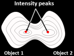    The object centers are defined as local intensity maxima in the smoothed image.

• Shape: For cases when there are definite indentations separating objects. The image is converted to black and white (binary) and the shape determines whether clumped objects will be distinguished. The declumping results of this method are affected by the thresholding method you choose.   This choice works best for objects that are round. In this case, the intensity patterns in the original image are largely irrelevant. Therefore, the cells need not be brighter towards the interior as is required for the Intensity option.

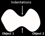    The binary thresholded image is distance-transformed and object centers are defined as peaks in this image. A distance-transform gives each pixel a value equal to the distance to the nearest pixel below a certain threshold, so it indicates the Shape of the object.

• Laplacian of Gaussian: For objects that have an increasing intensity gradient toward their center, this option performs a Laplacian of Gaussian (or Mexican hat) transform on the image, which accentuates pixels that are local maxima of a desired size. It thresholds the result and finds pixels that are both local maxima and above threshold. These pixels are used as the seeds for objects in the watershed.
• None: If objects are well separated and bright relative to the background, it may be unnecessary to attempt to separate clumped objects. Using the very fast None option, a simple threshold will be used to identify objects. This will override any declumping method chosen in the settings below.

• Intensity: Works best where the dividing lines between clumped objects are dimmer than the remainder of the objects.

  Technical description: Using the previously identified local maxima as seeds, this method is a watershed (Vincent and Soille, 1991) on the intensity image.

• Shape: Dividing lines between clumped objects are based on the shape of the clump. For example, when a clump contains two objects, the dividing line will be placed where indentations occur between the two objects. The intensity patterns in the original image are largely irrelevant: the cells need not be dimmer along the lines between clumped objects. Technical description: Using the previously identified local maxima as seeds, this method is a watershed on the distance-transformed thresholded image.
• Propagate: This method uses a propagation algorithm instead of a watershed. The image is ignored and the pixels are assigned to the objects by repeatedly adding unassigned pixels to the objects that are immediately adjacent to them. This method is suited in cases such as objects with branching extensions, for instance neurites, where the goal is to trace outward from the cell body along the branch, assigning pixels in the branch along the way. See the help for the IdentifySecondary module for more details on this method.
• None: If objects are well separated and bright relative to the background, it may be unnecessary to attempt to separate clumped objects. Using the very fast None option, a simple threshold will be used to identify objects. This will override any declumping method chosen in the previous question.

This setting, along with the Minimum allowed distance between local maxima setting, affects whether objects close to each other are considered a single object or multiple objects. It does not affect the dividing lines between an object and the background.

Please note that this smoothing setting is applied after thresholding, and is therefore distinct from the threshold smoothing method setting above, which is applied before thresholding.

The size of the smoothing filter is automatically calculated based on the Typical diameter of objects, in pixel units (Min,Max) setting above. If you see too many objects merged that ought to be separate or too many objects split up that ought to be merged, you may want to override the automatically calculated value.

Reducing the texture of objects by increasing the smoothing increases the chance that each real, distinct object has only one peak of intensity but also increases the chance that two distinct objects will be recognized as only one object. Note that increasing the size of the smoothing filter increases the processing time exponentially.

This setting, along with the Size of smoothing filter setting, affects whether objects close to each other are considered a single object or multiple objects. It does not affect the dividing lines between an object and the background. Local maxima that are closer together than the minimum allowed distance will be suppressed (the local intensity histogram is smoothed to remove the peaks within that distance). The distance can be automatically calculated based on the minimum entered for the Typical diameter of objects, in pixel units (Min,Max) setting above, but if you see too many objects merged that ought to be separate, or too many objects split up that ought to be merged, you may want to override the automatically calculated value.

The maxima suppression distance should be set to be roughly equivalent to the minimum radius of a real object of interest. Any distinct "objects" which are found but are within two times this distance from each other will be assumed to be actually two lumpy parts of the same object, and they will be merged.

Note that if you have entered a minimum object diameter of 10 or less, checking this box will have no effect.

References

- Malpica N, de Solorzano CO, Vaquero JJ, Santos, A, Vallcorba I, Garcia-Sagredo JM, del Pozo F (1997) "Applying watershed algorithms to the segmentation of clustered nuclei." Cytometry 28, 289-297. (link)
- Meyer F, Beucher S (1990) "Morphological segmentation." J Visual Communication and Image Representation 1, 21-46. (link)
- Ortiz de Solorzano C, Rodriguez EG, Jones A, Pinkel D, Gray JW, Sudar D, Lockett SJ. (1999) "Segmentation of confocal microscope images of cell nuclei in thick tissue sections." Journal of Microscopy-Oxford 193, 212-226. (link)
- Wählby C (2003) Algorithms for applied digital image cytometry, Ph.D., Uppsala University, Uppsala.
- Wählby C, Sintorn IM, Erlandsson F, Borgefors G, Bengtsson E. (2004) "Combining intensity, edge and shape information for 2D and 3D segmentation of cell nuclei in tissue sections." J Microsc 215, 67-76. (link)
See also IdentifySecondaryObjects, IdentifyTertiaryObjects, IdentifyObjectsManually and ClassifyPixels
Settings:
Select the input image
Select the image that you want to use to identify objects.
Name the primary objects to be identified
Enter the name that you want to call the objects identified by this module.
Typical diameter of objects, in pixel units (Min,Max)
This setting allows the user to make a distinction on the basis of size, which can
be used in conjunction with the
Discard objects outside the diameter range? setting
below to remove objects that fail this criteria.